

⏱️ Read Time:
Introduction
Natural language processing has undergone a structural paradigm shift driven by the development of transformer based neural network architectures. Traditional statistical natural language processing techniques and early deep learning models, such as recurrent neural networks and long short term memory networks, relied on task specific engineering for isolated applications like text categorization, named entity recognition, or basic sequence to sequence translation. These historical approaches struggled to maintain contextual awareness over long text sequences, often losing information across extended inputs due to sequential processing bottlenecks.
The introduction of the transformer architecture established a unified modeling mechanism capable of evaluating bidirectional or unidirectional context across extensive sequences in parallel. Contemporary large language models rely primarily on decoder only transformer architectures. By scaling these deep neural networks across massive corpora of unlabelled text, models learn language syntax, complex semantics, and world knowledge through the foundational task of next token prediction.
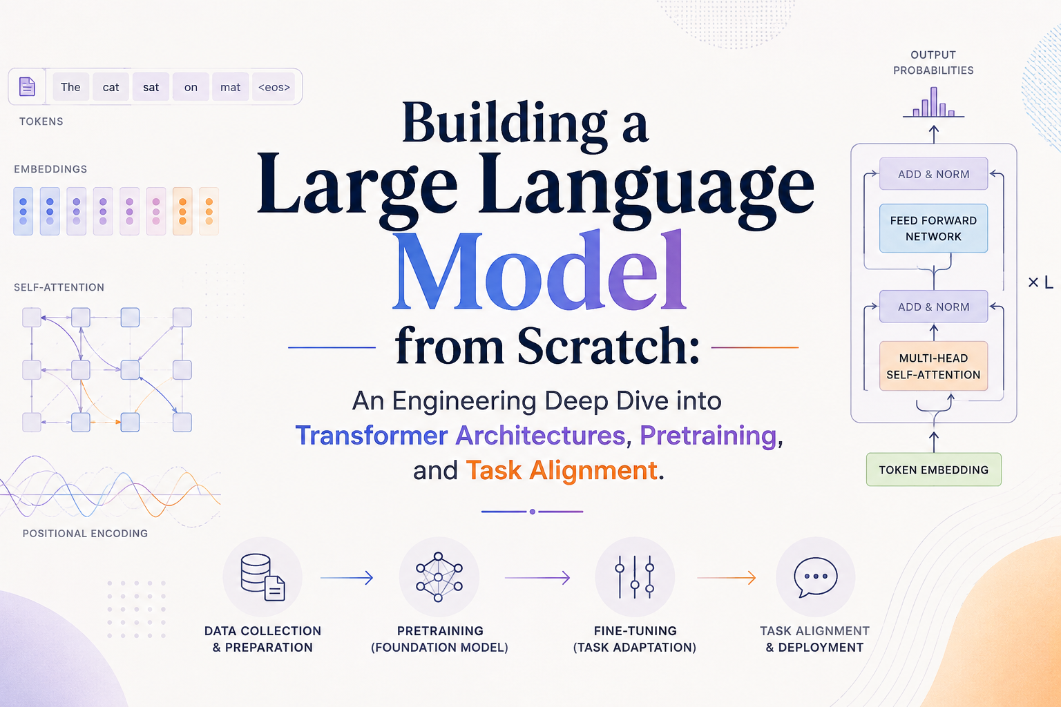
Building a functional large language model requires an end to end operational pipeline encompassing text tokenization, vector embedding construction, self attention mechanics, architectural backbone construction, pretraining, decoding optimization, and targeted task alignment. Understanding each stage at a mechanistic level enables engineers to construct, optimize, and deploy specialized language architectures tailored to specific privacy, efficiency, or domain requirements.
Data Preparation, Tokenization, and Embedding Construction
Deep neural networks are inherently numeric processing systems that cannot parse raw textual characters directly. Transforming unstructured natural language into a numerical format compatible with backpropagation requires structured data pipeline engineering. This phase encompasses text segmentation, vocabulary construction, token to vector mapping, and positional encoding.
Tokenization Schemes and Byte Pair Encoding
Tokenization is the initial preprocessing phase wherein continuous text is segmented into smaller, discrete units called tokens. Tokens can represent whole words, subwords, or individual characters, including punctuation marks. Simple whitespace or punctuation based splitting strategies fail to handle rich vocabularies efficiently, leading to excessively large vocabulary sizes or frequent out of vocabulary tokens that must be mapped to generic unknown markers.
To solve vocabulary constraints while ensuring complete textual coverage, modern language models employ subword tokenization algorithms, most notably Byte Pair Encoding. Byte Pair Encoding iteratively constructs a fixed size vocabulary by analyzing character frequency and merging the most frequent adjacent character or subword pairs across a training corpus.
The primary advantage of subword tokenization via Byte Pair Encoding lies in its ability to decompose unfamiliar or rare words into recognizable subword fragments or individual characters. Consequently, a Byte Pair Encoding tokenizer can process any arbitrary text sequence without requiring dedicated markers for unknown words. Standard implementation pipelines, such as those utilized in Generative Pre trained Transformer style architectures, maintain a fixed vocabulary size, mapping each unique subword token to an integer token identifier.
Contextual Data Sampling and Positional Encodings
Once text is converted into a sequence of integer token identifiers, it must be structured into training pairs suitable for self supervised learning. Pretraining relies on next token prediction, where the neural network accepts an input sequence and attempts to predict the sequence shifted forward by a single position.
A sliding window data sampling strategy is utilized to extract fixed length input chunks from continuous tokenized datasets. Given a defined context window length and a stride parameter, the sampling algorithm extracts input feature tensors and corresponding target tensors where target tokens match the input tokens shifted by one step into the future. The stride parameter determines the degree of overlap between consecutive training samples, balancing computational throughput and data variance.
To feed discrete token identifiers into the neural network, an embedding layer maps each integer identifier to a continuous dense vector of fixed hidden dimension. This lookup matrix translates categorical identifiers into high dimensional representation space. The initial weights are distributed randomly and subsequently updated during model optimization.
A fundamental characteristic of the self attention mechanism is its permutation invariance. Unlike recurrent neural networks, self attention processes all sequence positions simultaneously without an inherent sense of temporal order. To supply sequence order information, absolute positional embeddings are constructed. These positional vectors share the exact same hidden dimensionality as the token embeddings and are added directly elementwise to the token embedding vectors. Conceptually, the final input representation equals the sum of the token vector and its positional vector. This combined representation carries both the semantic identity of the token and its precise sequential coordinate within the input context window.
Mechanics of Self Attention Systems
The self attention mechanism represents the algorithmic core of the transformer architecture. It allows the neural network to dynamically weigh the contextual relevance of every token in a sequence relative to all other tokens, forming contextualized representations.
Query, Key, and Value Transformations
Scaled dot product self attention projects input sequence vectors into three distinct vector spaces using trainable weight matrices. Input representations are transformed into three specialized representations for each token:
- Query: Represents the current token seeking contextual information from other tokens in the sequence.
- Key: Represents the indexing features of all tokens used for matching against incoming queries.
- Value: Represents the actual contextual content that is aggregated to form the final updated representation.
The logical alignment between a query vector and a key vector is quantified by calculating their vector dot product. High dot products indicate strong semantic or syntactic similarity between corresponding tokens. To prevent dot product magnitudes from growing excessively large in high dimensional feature spaces, which causes the Softmax function to saturate and yield vanishing gradients during backpropagation, inner products are scaled down by the square root of the key feature dimension. Normalizing these values using the Softmax function produces attention probability weights, which are then used to compute a weighted sum of the value vectors.
Causal Masking and Multi Head Parallelism
In decoder only autoregressive language models, the network must predict future tokens without accessing subsequent context within the training sequence. Unmasked self attention would allow the model to access future target tokens directly, invalidating the learning objective.
To preserve temporal causality, causal masking is applied to raw attention scores prior to evaluating the Softmax step. Masking sets all attention scores for future positions to negative infinity. Because the Softmax transform maps negative infinity values to zero, future tokens receive zero attention weight. This guarantees that the representation for a token at position t depends strictly on tokens at positions up to and including position t.
To expand model capacity to focus on multiple contextual relationships concurrently, multi head attention is employed. Instead of computing a single attention function across the full feature space, query, key, and value projections are split into multiple independent channels called attention heads. Each head computes scaled dot product attention independently in parallel, capturing distinct syntactic and semantic relationships. Outputs from all attention heads are concatenated along feature channels and projected back to the primary hidden dimension using an output linear transformation.
Architectural Assembly of the Transformer Backbone
A complete Generative Pre trained Transformer style decoder model integrates multi head self attention modules within repeated transformer blocks, complemented by normalization routines, activation functions, and residual connections.
Normalization Layers and Non Linear Activations
Training deep neural networks with many layers can become numerically unstable due to internal covariate shift, where activation distributions fluctuate across iterations. Layer Normalization adjusts neural network activations to maintain zero mean and unit variance across the feature dimension for each sample independently. Trainable scale and shift parameters allow the network to preserve representational capacity while stabilizing feature distributions. Modern transformer variants utilize Pre Layer Normalization placement, applying normalization prior to entering multi head attention and feed forward modules rather than post application. This structural adjustment substantially improves training convergence stability in deep architectures.
Within feed forward submodules of each transformer block, nonlinear activation functions expand model expressivity. Contemporary language models prefer the Gaussian Error Linear Unit over traditional activation choices. The Gaussian Error Linear Unit scales inputs probabilistically based on the Gaussian cumulative distribution function, providing a smooth curve that retains small negative gradient information and enhances feature learning.
Feed Forward Networks and Residual Shortcuts
Each transformer block incorporates a position wise Feed Forward Network following the attention submodule. The Feed Forward Network consists of two linear transformations separated by a Gaussian Error Linear Unit activation. The first linear layer expands hidden feature dimensionality fourfold, providing higher dimensional capacity for pattern extraction. The second linear layer projects expanded features back down to baseline hidden dimension.
To prevent the vanishing gradient problem across deep stacks of transformer blocks, residual shortcut connections bypass each major submodule. Unmodified module inputs are added directly to submodule outputs. These skip pathways create an unimpeded channel for gradient flow during backpropagation, enabling stable optimization across deep networks.
The structural data flow within a single block begins with an input tensor entering Layer Normalization. The normalized tensor passes into masked multi head attention, followed by dropout. The result is added to the original input tensor via a residual shortcut connection. This combined tensor passes through a second Layer Normalization step, enters the position wise Feed Forward Network, passes through dropout, and is added to intermediate features through a second residual shortcut connection.
Pretraining Dynamics, Loss Evaluation, and Decoding Strategies
Pretraining constructs a foundational language model from unlabelled text corpora through self supervised next token prediction. Computational efficiency and output stability depend on optimized training loops, evaluation metrics, and controlled generation sampling.
Objective Functions and Pretraining Optimization
During pretraining, the model processes sequence inputs and generates raw output scores, known as logits, for every token in the vocabulary at each sequence position. Logits are evaluated against target token identifiers using categorical Cross Entropy Loss.
Cross Entropy Loss measures the divergence between predicted probability distributions and actual target token sequences. In language modeling, Perplexity is reported alongside loss as an intuitive performance metric. Perplexity equals the exponentiated cross entropy loss. Conceptually, perplexity measures model uncertainty as the effective number of uniform choices among vocabulary tokens at each prediction step.
Model optimization typically employs the AdamW optimizer, an extension of Adam that decouples weight decay from gradient updates. Training schedules incorporate a linear learning rate warmup phase followed by cosine decay that gradually reduces learning rate toward a minimum threshold. Gradient clipping caps maximum gradient norms to prevent parameter instability caused by exploding gradients.
Stochastic Decoding and Output Controls
Generating text involves iterating next token predictions, appending predicted tokens back to input context sequentially. Selecting tokens strictly via greedy decoding, which always chooses the highest probability token, leads to repetitive outputs and looping text patterns.
Stochastic decoding techniques introduce controlled variance and natural fluency:
- Temperature Scaling: Temperature controls distribution entropy. Dividing logits by a temperature value prior to Softmax alters probabilities. Setting temperature below 1.0 sharpens probabilities toward top candidates for confident output. Setting temperature above 1.0 flattens distribution spread to foster creative generation.
- Top k Sampling: Top k sampling truncates vocabulary candidates at each step, restricting sampling to the k most probable tokens. Logits below the kth rank are masked to negative infinity prior to Softmax, eliminating nonsensical tail tokens.
Downstream Fine Tuning and Domain Adaptation
A foundation model trained solely on next token prediction operates as a general text completion engine. Adapting it for targeted practical applications requires fine tuning methodologies categorized into classification adaptation and instruction alignment.
Task Specific Classification Heads
For classification tasks such as sentiment analysis or spam detection, the foundation model vocabulary output layer is replaced by a classification head with output width matching target class counts. Because causal attention aggregates context from preceding positions, the final vector representation at the final sequence token index contains accumulated contextual information across the input. Classification models extract this final hidden state and project it through the classification head to compute class probabilities.
| Architectural Component | Pretraining Configuration | Classification Adaptation Configuration |
| Input Interface | Variable length token sequences | Padded or truncated sequence batches |
| Attention Mechanism | Causal multi head self attention | Causal multi head self attention |
| Extracted Feature Representation | Full matrix of hidden states | Final token hidden vector |
| Output Head Dimension | Vocabulary dimension | Class count dimension |
| Primary Loss Function | Next token Cross Entropy Loss | Categorical Class Cross Entropy Loss |
During classification fine tuning, parameter updates can be applied across the entire network or restricted to the output head and final transformer blocks, reducing training costs while preserving baseline language representations.
Supervised Instruction Fine Tuning and Parameter Efficiency
Supervised Instruction Fine Tuning transforms a foundational base model into an interactive assistant capable of answering questions, summarizing, and following complex human prompts. Supervised Instruction Fine Tuning relies on curated instruction datasets formatted using structured prompt templates. Formatting structures organize data into distinct components, specifying task instructions, optional context, and target responses.
During training, concatenated instructions and responses are processed by the network. Loss computation can be restricted strictly to response tokens by masking prompt positions, instructing the loss function to ignore instruction tokens.
To optimize computational efficiency, Parameter Efficient Fine Tuning frameworks like Low Rank Adaptation (LoRA) are integrated. Low Rank Adaptation freezes primary weight matrices and injects pairs of low rank decomposition matrices. Low Rank Adaptation drastically reduces trainable parameter counts without significant degradation in task performance.
Structural Comparison of Model Configurations
Transformer architectural principles scale predictably across parameter scales. Primary structural dimensions across standard model scales illustrate relationships between depth, feature dimensions, and parallel heads.
| Model Configuration Variant | Total Parameters | Hidden Dimension | Transformer Blocks | Attention Heads | Context Length |
|---|---|---|---|---|---|
| GPT 2 Small | 124 Million | 768 | 12 | 12 | 1,024 |
| GPT 2 Medium | 355 Million | 1,024 | 24 | 16 | 1,024 |
| GPT 2 Large | 774 Million | 1,280 | 36 | 20 | 1,024 |
| GPT 2 XL | 1.558 Billion | 1,600 | 48 | 25 | 1,024 |
| GPT 3 Base | 175 Billion | 12,288 | 96 | 96 | 2,048 |
Recommended Readings
- Raschka, S. (2025). Build a Large Language Model (From Scratch). Manning Publications.
- Huyen, C. (2022). Designing Machine Learning Systems: An Iterative Process for Production Ready Applications. O’Reilly Media.
- Tunstall, L., von Werra, L., & Wolf, T. (2022). Natural Language Processing with Transformers: Building Language Applications with Hugging Face (Revised ed.). O’Reilly Media.
Frequently Asked Questions
Why is causal masking necessary in decoder only language models?
Causal masking prevents a model from accessing information from future positions during self supervised training. In autoregressive text generation, the network must predict the next token relying strictly on current and preceding contexts. Without causal masking, self attention would allow tokens to attend to subsequent target tokens, allowing the network to memorize future inputs rather than learning underlying contextual dependencies.
How does Byte Pair Encoding handle words that were not present in the training data?
Byte Pair Encoding avoids out of vocabulary issues by operating at subword and character levels. If an unseen word is encountered during inference, the Byte Pair Encoding tokenizer breaks the term down into its constituent subword segments or individual characters that exist within its pre built vocabulary. In extreme cases, any unknown string is reduced to base character representations, guaranteeing that all input text can be processed without using generic unknown tokens.
What is the purpose of scaling dot products in self attention systems?
In scaled dot product attention, query and key feature vectors are multiplied together. As hidden feature dimensions increase, dot product values grow larger. Large values push the Softmax function into regions with extremely small gradients, leading to vanishing gradient problems during backpropagation. Scaling dot products down maintains stable variance, keeping Softmax outputs within regions that provide meaningful gradients for optimization.
How do residual shortcut connections assist in training deep transformer models?
Residual shortcut connections add the input tensor of a module directly to its output tensor. During backpropagation, this structural design allows gradients to flow directly through addition operations without encountering matrix multiplication scaling at every layer. Consequently, skip connections mitigate vanishing and exploding gradient phenomena, allowing neural networks with dozens of transformer layers to converge stably.
What is the fundamental difference between pretraining and instruction fine tuning?
Pretraining is a self supervised process where a language model learns general language patterns, syntax, and world knowledge by predicting the next token across massive, unlabelled text datasets. Instruction fine tuning is a supervised process that takes a pretrained foundation model and further updates its weights using structured instruction response pairs. This fine tuning process aligns model outputs with human conversational expectations, transitioning it from a basic text completion engine into an instruction following assistant.
Conclusion
The construction of modern large language models represents a systematic integration of data processing pipelines, attention mechanics, and modular neural architectures. Beginning with raw textual processing, byte pair encoding algorithms resolve vocabulary boundary constraints, allowing continuous text to be encoded as numeric input streams. Positional encodings augment high dimensional token embeddings, restoring sequence order information to permutation invariant self attention operations.
At the architectural core, multi head causal self attention enables neural networks to compute contextualized feature representations while preserving strict autoregressive boundaries through score masking. Pre Layer Normalization, Gaussian Error Linear Unit activations, and residual skip connections stabilize optimization dynamics, permitting deep architectures to be trained effectively.
Finally, foundational pretraining equips models with broad linguistic and semantic representations that can be adapted efficiently. Whether deploying specialized classification heads or applying parameter efficient instruction alignment via Low Rank Adaptation, structured fine tuning converts raw completion engines into practical natural language systems tailored for real world production tasks.













Leave a Reply